
My Learning Reflections about Optimizing Neural Networks (Part 3): Navigating Activation Functions, Gradient Flow, and Data & Compute Requirements

Editor’s Note: This is Part 3 of a multi-part series covering my learning reflections and industry validations about neural network optimization. The series draws from Cornell University‘s eCornell “Designing and Building AI Solutions” program (instructed by Lutz Finger). Each article examines specific optimization aspects alongside market observations, building toward comprehensive understanding.
The concepts explored here build directly on Part 2. Understanding why the chain rule’s multiplicative nature makes activation function choice so critical provides the bridge between mathematical theory and practical implementation. This article also expands into data requirements and computational trade-offs, themes introduced in Part 2 that warrant deeper exploration given the massive infrastructure investments now defining the AI industry.
What I have been up to: I continue building the semantic layer and LLM component for my personal News Analyst application. This locally deployed system transforms high-volume, fast-moving AI news into structured metadata for deeper pattern analysis. Truly exciting times for personal AI solutions (robot-butler aside)!
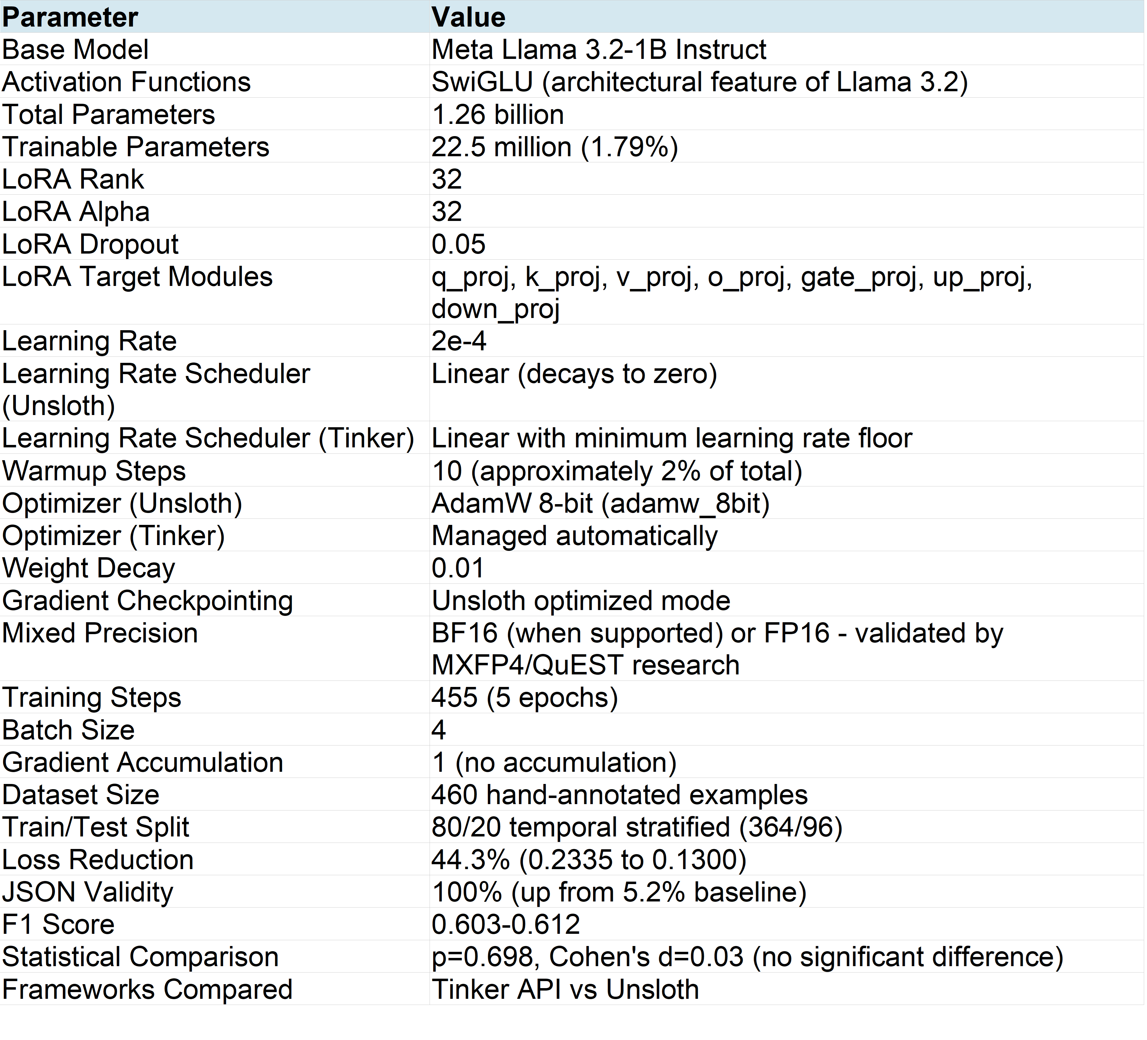
My v2 llama-tinker-lora-news-enhancer project demonstrates gradient flow and data management principles in practice. The project fine-tunes the relatively smaller Meta Llama 3.2-1B model using LoRA (rank 32) on 364 training examples with an 80/20 temporal stratified split. I compared two frameworks: Thinking Machines Lab’s Tinker API and Unsloth AI’s optimization library. Both single-run fine-tuning processes achieved 100% JSON validity and F1 scores of 0.603-0.612 (vs. Base Model 5.2% JSON validity, F1 score of 0.396), validating the optimization principles covered in this article.
Project repositories:
v2 AI Industry News Enhancer (Production): GitHub | Hugging Face
v1 AI Related News Enhancer (Proof of Concept): GitHub | Hugging Face
The Meta Llama 3.2-1B base model employs SwiGLU activation functions, which directly connects to this article’s theme. SwiGLU represents a significant advancement over classical activation functions like ReLU. While ReLU suffers from the “dying neuron” problem where neurons permanently deactivate upon receiving negative inputs, SwiGLU combines the Swish activation with a gating mechanism. This gated approach provides smoother gradients and allows the network to learn which information to propagate. Unlike sigmoid and tanh, which compress values into narrow ranges and cause vanishing gradients (where gradients become so small during backpropagation that the network stops learning), SwiGLU maintains effective gradient flow throughout deep architectures. My fine-tuning work inherited these gradient flow benefits directly from the base model’s architecture.
Following my exploration of backpropagation mathematics and gradient optimization in Part 2, I now turn to activation functions, data requirements, and computational trade-offs. These critical architectural choices directly impact gradient flow and model performance. As I continue reflecting on my 5-month journey through Cornell University‘s eCornell “Designing and Building AI Solutions” certificate program instructed by Lutz Finger, this segment of the fourth module revealed how activation function selection can make the difference between a network that learns effectively and one that suffers from vanishing gradients or dying neurons. The module also emphasized the fundamental challenge of balancing data volume, model complexity, and computational efficiency.
Each optimization decision represents a strategic design choice aligned with specific objectives. Selecting activation functions, configuring gradient flow, and allocating data and compute resources are not purely technical exercises. They require alignment with personal, business, or societal objective functions while maintaining consistency with external market conditions and internal execution capabilities. Every choice involves trade-offs: optimizing one dimension often incurs opportunity costs in others. Understanding these trade-offs enables practitioners to establish differentiated positions rather than investing capital and resources across all dimensions which brings an undifferentiated “middle of the pack” position that excels at nothing.
Why Activation Function Choice Is Critical
Part 2 covered backpropagation and the vanishing gradient problem. Here is the key insight that connects those concepts to this article: during backpropagation, gradients are multiplied at each layer by the activation function’s derivative. Sigmoid derivatives are at most 0.25. Multiply 0.25 by itself across 100 layers and you get 10⁻⁶¹, a number so small the network stops learning. This cascade effect explains why activation function choice determines whether deep networks can train at all. Modern activation functions like SwiGLU address this by maintaining healthier gradient magnitudes throughout the network.
Modern Activation Functions: Beyond Classical Approaches
Modern activation function research has evolved beyond classical sigmoid, tanh, and ReLU functions. Contemporary neural architectures increasingly adopt variants like SwiGLU (used in Llama models), GELU (Gaussian Error Linear Unit), and Mish. These offer improved gradient flow characteristics and training stability. These modern activation functions address limitations of classical approaches while maintaining computational efficiency.
1) GLU-Based Activation Functions Become Industry Standard
SwiGLU has gained widespread production adoption across major language models. Introduced by Noam Shazeer in his 2020 paper “GLU Variants Improve Transformer,” SwiGLU combines the Swish activation with a gating mechanism to provide smoother gradients. Meta’s Llama 3.1 and 3.2 models use SwiGLU in their feed-forward layers to improve training stability and efficiency. Google’s Gemini architecture also incorporates gated linear units. This industry-wide adoption validates that gated activation mechanisms provide meaningful improvements over simpler alternatives.

Newer activation functions continue pushing the boundaries of efficiency and performance. The xIELU activation function, introduced by Huang (2024), gained traction in 2025 when Switzerland (Swiss AI Initiative)’s Apertus models adopted it as a core architectural innovation, demonstrating improved training stability at the 70B scale. This represents Switzerland’s first large-scale open, multilingual language model, which is trained on 15 trillion tokens across more than 1,000 languages (including many languages that have so far been underrepresented in LLMs, such as Swiss German, Romansh, and many others). Apertus (Meaning “open” in Latin) is intended as a building block for developers and organizations for future applications such as chatbots, translation systems, or educational tools. Research into activation function combinations continues to grow. New hybrid approaches such as S3 (Sigmoid-Softsign) and S4 (Kavun, 2025) combine characteristics from different functions, using sigmoid for negative inputs and softsign for positive inputs, to optimize both forward propagation and gradient flow.
2) Recent Novel Gradient Flow Architectures Address Vanishing Gradients
Gradient Networks (GradNets) directly parameterize gradients of function classes: Introduced in 2024, these architectures ensure learned functions are true gradient fields. GradNets avoid common pitfalls that cause training instabilities. They guarantee the existence of valid antiderivative functions. This approach represents a fundamental shift from traditional activation-based gradient management.
The Scaling with Gradient Grouping (SGG) optimizer dynamically clusters gradient statistics within each layer: SGG applies group-specific scaling to calibrate learning rates. This approach yields average improvements of 5% on vision tasks and 2% on language tasks compared to Adam. The technique addresses the heterogeneous gradient magnitudes that emerge in deep architectures.
Meta’s Dynamic Tanh (DyT) research challenges a decade of neural network orthodoxy: Meta’s FAIR team (including Yann LeCun) demonstrated (June 2025) that Transformers can match or exceed performance without traditional normalization layers. DyT replaces layer normalization with DyT(x) = tanh(αx), where α is a learnable parameter. This simple element-wise operation mimics the S-shaped input-output mappings that layer normalization naturally produces, squashing extreme activation values while preserving linear behavior for typical inputs. Remarkably, LLaMA models up to 70B parameters trained with DyT achieved equivalent performance to RMSNorm counterparts. This finding suggests gradient stabilization techniques continue evolving beyond established norms, potentially enabling architectural simplification for specialized hardware deployment.
3) LoRA-Specific Activation Strategies Enhance Fine-Tuning
SineLoRA applies sinusoidal activation to LoRA adapters to enhance expressivity under quantization. This method achieves up to 66% memory reduction with similar or improved performance compared to standard LoRA. The sinusoidal activations help LoRA adapters maintain gradient flow even with aggressive quantization. This directly addresses the memory constraints that make LoRA attractive for consumer hardware.
MiLoRA focuses on updating only the minor singular components of weight matrices during fine-tuning. This approach preserves pretrained knowledge more effectively. MiLoRA consistently outperforms standard LoRA across multiple model sizes and tasks. The technique demonstrates that gradient pathway design within adapters significantly impacts fine-tuning outcomes.
The Data Hunger Phenomenon and Diminishing Returns
Neural networks require substantially more data than traditional machine learning approaches due to their parameter complexity. The eCornell program illustrated this progression clearly. From logistic regression to decision trees to neural networks, each step increases the ability to learn non-linear patterns but demands dramatically more training data. This “data hunger” stems from the sheer number of parameters requiring calibration. In a neural network, each connection between neurons has a weight that must be learned from data, and each neuron has a bias term. A complex network with multiple layers and hundreds of neurons needs far more training examples to capture complex patterns without overfitting.
Diminishing returns apply to both data volume and model complexity. Through the eCornell program, I drove home the understanding that adding more data or network layers eventually yields minimal learning or performance improvements. By evaluating training, validation and test performance across epochs, we can identify when additional model complexity, compute or data reaches the “plateau” and stops providing meaningful value. The program emphasized that an efficient approach starts with simpler architectures and gradually increases complexity while monitoring performance. This relationship works in both directions: More complex datasets may benefit from more complex neural network architectures, though this is not universal. If you recall my reflections in previous articles and earlier passages, simpler model architectures may even achieve comparable performance at lower (if not similar) cost. For example, my v2 AI-Related News Enhancer project (v2 llama-tinker-lora-news-enhancer) was deliberately constrained by costs, hardware and dataset.
Optimal Data Allocation: The 70/15/15 and 80/10/10 Principles
The eCornell program exercises reinforced a critical principle in neural network training: Finding the optimal balance in data allocation across training, validation, and test sets. AI practitioners typically split datasets into three subsets: a training set (used to teach the model), a validation set (held out from training to evaluate performance and tune hyperparameters during development), and a test set (completely reserved until the end for unbiased final assessment). Common ratios include 70/15/15 or 80/10/10 for training/validation/test splits, with the exact proportions determined by dataset size/volume, size, model complexity, domain requirements or other strategic design considerations.
Smaller datasets require larger validation and test sets to ensure reliable estimates. Larger datasets can allocate proportionally less to validation and testing. This three-way separation ensures models learn generalizable patterns rather than merely memorizing patterns in data. Through hands-on experimentation, I learned that model performance follows a characteristic curve marked by steady improvements with additional training data up to an optimal point, followed by diminishing returns or even performance degradation.
Cross-Validation and Temporal Validation Techniques
Cross-validation provides a robust framework for assessing model generalization and determining data sufficiency. The eCornell program taught us to divide data into k folds, training on k-1 folds and testing on the remaining fold, repeating this process k times. This technique ensures models perform consistently across different data subsets, providing confidence that the network will generalize well to unseen data rather than simply memorizing training examples. In practice, k=5 or k=10 are common choices that balance computational cost with robust validation.
I learned to recognize that standard k-fold cross-validation has limitations for time-series or temporal data. Random shuffling can introduce look-ahead bias. In these cases, models inadvertently train on “future” data to predict the past, presenting unrealistically exceptional model performance. Financial applications and quant hedge funds must use walk-forward validation that strictly respects the chronological order of data, always training on historical data and testing on subsequent periods. This distinction between spatial and temporal validation strategies proves essential for understanding real-world model deployment.
Managing Computational Complexity and Trade-offs
Computational complexity scales dramatically with network architecture. As explored in Part 2, even a modest MNIST classifier requires optimizing hundreds of parameters, and each parameter requires gradient computation during every training iteration. The eCornell program exercises demonstrated that adding architectural complexity (e.g., more layers, more neurons/nodes) does not always yield proportional performance gains, yet it consistently increases computational demands.
This relationship between architectural complexity and compute requirements plays out at industry scale: Epoch AI (May 2025) projects that the number of notable AI models exceeding 10²⁶ FLOP will grow from ~10 models by 2026 to 200+ models by 2030, with hardware acquisition costs for the largest training runs potentially reaching $200 billion to $1 trillion by decade’s end. Managing the sheer computational complexity at scale requires specialized hardware like NVIDIA GPUs and Google TPUs, which optimize the intensive multiply-accumulate operations at the core of neural network training.
Yet, the eCornell program exercises revealed a crucial insight: Adding network architectural complexity does not always translate to proportional performance improvements. In one exercise, Lutz Finger demonstrated that a two-layer network with 128 and 64 neurons performed marginally better than a simpler 65-neuron network. Yet, the minimal gains relative to the increased computational needs showed we might be approaching the point of diminishing returns or even overfitting. The relationship between architectural complexity and performance proved nonlinear. Single-layer networks frequently achieved performance within a few percentage points of far more complex multi-layer architectures.
Recent Industry Developments: Massive Infrastructure Investments
The year 2025 sees unprecedented investment in AI infrastructure, validating that compute availability remains a critical constraint. Building on the infrastructure landscape covered in Part 1 (including OpenAI’s $300 billion Oracle agreement), the competitive intensity has only accelerated. Anthropic committed to purchasing $30 billion of Azure compute capacity from Microsoft, contracting for additional capacity up to 1 gigawatt (GW). These commitments reflect how artificial intelligence has shifted into a new phase centered on long-term infrastructure positioning rather than just model releases.
Meta was tracked at $75.5 billion in infrastructure deals between September and October 2025 alone. This hit the highest capital expenditure ratio (37% of revenue or sales) in the company’s history to finance superintelligent AI systems. Meta’s plans include building data centers covering significant portions of Manhattan’s footprint. The company projects capital expenditures for 2025 to reach between $66 billion and $72 billion, representing an increase of approximately $30 billion year-over-year. Meta anticipates a similarly substantial surge in spending on AI infrastructure in 2026.
These massive infrastructure investments validate the eCornell program’s emphasis on computational efficiency as a critical constraint in neural network design. The competition extends beyond cloud infrastructure to custom chip development. The race to secure compute capacity has become as strategically important as model development itself. Research from the AI research organization METR (March 2025) shows that AI task-completion capabilities are doubling approximately every seven months, validating the urgency of these infrastructure investments while also demonstrating that even massive compute cannot overcome all capability limitations.
Low-Precision Computation Complements Infrastructure Scale
Beyond massive infrastructure investments, architectural efficiency through low(er)-precision computation has become equally critical. This validates my choice of mixed precision (BF16/FP16) training in the v2 project. OpenAI’s MXFP4 data type (August 2025) demonstrates how quantization can cut LLM inference costs by 75%, enabling 120 billion parameter models to fit on 80GB VRAM hardware. Research like QuEST (February 2025) has achieved stable training with just 1-bit weights and activations, pushing the boundaries of memory-efficient computation. These offer more variable options whereby precision optimization (for lower precision) require strategic decisions for efficiency gains, as with raw compute scaling.
Federated Computing Addresses Data Sovereignty Challenges
Federated computing enables AI model training without moving sensitive data, addressing the data access bottleneck in healthcare and life sciences. German startup Apheris raised $20.8 million in Series A funding to power federated data networks. Their Compute Gateway, which is a software agent that serves as a gateway between local data and AI models, allows researchers to run AI models on clinical datasets without transferring the underlying data. Customers include Roche, Johnson & Johnson, and several leading hospitals. Their approach aims to resolve this problem statement: 97% of all healthcare data remains completely unused because it is siloed across organizations and cannot be shared due to regulatory and commercial sensitivity.
The AI Structural Biology (AISB) Consortium demonstrates federated computing at scale in an organization structure. Members including AbbVie, Boehringer Ingelheim, Johnson & Johnson, and Sanofi collaborate on AI-driven drug discovery using Apheris’s Compute Gateway. Beyond the Consortium’s strategic partnership and its contractual obligations, member companies can customize AI drug discovery models on proprietary pharma data while preserving data privacy. This represents a solution to the data hunger problem: rather than centralizing more data, federated approaches bring computation to distributed data sources.
Practical Application: Data Management in My v2 Project
Building on the v2 AI Industry News Enhancer (v2 llama-tinker-lora-news-enhancer) project introduced in Part 2, I gained hands-on experience with data allocation and validation strategies. I hand-annotated 460 AI news examples, inspecting each one individually to ensure data quality. This manual annotation process, while time-consuming, ensured that training labels accurately reflected the task requirements. The project evolved from v1’s proof-of-concept with 101 examples to v2’s production-ready dataset of 460 examples, demonstrating the principle that dataset expansion should be deliberate rather than arbitrary.
I implemented an 80/20 temporal stratified split to respect the chronological nature of news data. Rather than random shuffling, I extracted the month from each article’s email date and split proportionally within each month. This approach prevents look-ahead bias where the model might learn patterns from “future” articles to predict earlier ones. The final split produced 364 training examples and 96 test examples, with temporal distribution preserved across both sets. This validates the eCornell program’s emphasis on validation strategy matching the deployment context.
Balancing Data Volume Against Quality and Annotation Cost
The 460-example dataset represented a deliberate balance between coverage and annotation effort. I had access to over 7,000 raw news items from my data pipeline, but hand-annotating all of them would have been impractical. Instead, I focused on achieving sufficient diversity across relevance scores (1-10 scale), news categories, and time periods. The resulting dataset proved sufficient for the task: both fine-tuned models achieved 100% JSON validity and F1 scores above 0.60, suggesting that additional data may yield diminishing returns.
As a recap from Part 2, baseline comparison validated that fine-tuning was essential, not optional. The untrained Llama 3.2-1B baseline achieved only 5.2% JSON validity, F1 score of 0.396, and MAE of 6.98. The fine-tuned models achieved 100% JSON validity and F1 scores of 0.603-0.612. This represents a 19-times improvement in JSON validity. The relevance score error dropped by nearly 5 times. This stark contrast demonstrates that architectural optimization through LoRA fine-tuning enables new capabilities that the base model cannot achieve through prompting alone.
Gradient Flow Configuration: Framework Comparison
The Llama 3.2-1B base model uses SwiGLU activation functions throughout its architecture. This is not something I configured during fine-tuning. SwiGLU is an architectural feature ‘baked’ into the model by Meta. Neither Unsloth nor Tinker modifies the base model’s activation functions. My fine-tuning work operated within the gradient flow characteristics established by this architectural choice. I cannot isolate SwiGLU’s specific contribution to my results without comparative experiments using different base architectures.
Unsloth provided full control over gradient-related hyperparameters. I configured the AdamW optimizer with 8-bit quantization (adamw_8bit), which maintains per-parameter adaptive learning rates based on gradient history. I set weight decay to 0.01 for L2 regularization, which adds a penalty term that affects gradient updates. The learning rate started at 2e-4 with a linear decay schedule and 10 warmup steps, allowing gradient statistics to stabilize before applying the full learning rate.
As a managed service, Thinking Machines Lab’s Tinker API managed several gradient-related settings automatically. The optimizer choice, gradient accumulation, and gradient clipping were not exposed for configuration. Analysis of Tinker’s training logs revealed the scheduler behavior. The learning rate decayed from 0.0002 to approximately 0.000058 over 455 steps. This final value (roughly 29% of initial) indicates a minimum learning rate floor rather than decay to zero. For Tinker API, training logs confirm linear decay behavior (verified by analyzing step-by-step learning rate values). For Unsloth, linear decay was configured in the TrainingArguments to match Tinker’s behavior, with both frameworks using a minimum learning rate floor of approximately 29% of the initial value. This difference in control levels has implications for reproducibility and debugging.
To ensure a fair comparison, we controlled all parameters that both frameworks expose: base model (Llama 3.2-1B), precision (16-bit), learning rate (2e-4), LoRA configuration (rank=32, alpha=32, dropout=0.05), target modules (all seven weight matrices), batch size (4), epochs (5), and identical training/test splits. Parameters managed internally by Tinker (e.g. optimizer, weight decay, warmup schedule) could not be directly matched, which itself illustrates the managed-versus-manual tradeoff central to choosing between these frameworks.
LoRA Configuration: Shaping Gradient Pathways
LoRA creates low-rank adapter matrices through which gradients flow during fine-tuning: I configured LoRA rank at 32 with alpha set to 32 (matching rank is standard practice). The rank determines the dimensionality of the gradient pathway. Lower ranks constrain gradient updates to a smaller subspace. Higher ranks allow more expressive updates but increase memory requirements and risk overfitting. LoRA dropout at 0.05 randomly zeros adapter outputs during training, providing regularization that prevents overfitting to training data patterns.
Target module selection determines which weight matrices receive gradient updates: I configured LoRA to adapt all major weight matrices: q_proj, k_proj, v_proj, o_proj (attention) and gate_proj, up_proj, down_proj (feed-forward). This comprehensive targeting ensures gradients can update representations throughout the network. Limiting to attention-only modules would constrain the model’s ability to learn task-specific transformations in the feed-forward layers where much of the computational work occurs.
Observed Training Dynamics: Attributing Results Accurately
The smooth loss reduction I observed resulted from the full system, not any single component: Training loss decreased 44.3% across 455 steps (from 0.2335 to 0.1300 in Unsloth’s cross-entropy metric). This convergence resulted from the combined effect of SwiGLU activation functions (inherited), AdamW optimizer with adaptive learning rates (configured), learning rate warmup and decay (configured), gradient checkpointing (configured), and response-only training (configured). Attributing the smooth convergence to any single factor would be technically inaccurate.
Both frameworks achieved statistically equivalent results despite different gradient configurations: Tinker and Unsloth produced models with p=0.698 and Cohen’s d=0.03, indicating no significant performance difference. This statistical equivalence suggests that SwiGLU architecture provides sufficient gradient stability that specific optimizer and scheduler choices become less critical. The absence of gradient pathologies confirmed that my configurations were appropriate. Neither framework showed loss spikes (exploding gradients) or premature plateaus (vanishing gradients).
Looking Ahead: Strategic Design Decisions in Neural Network Optimization
The optimization decisions explored in this article, including activation functions, gradient flow, and data and compute allocation, are fundamentally strategic choices, not merely technical configurations. Each decision requires alignment with an objective function (personal learning, business ROI, or societal impact) while maintaining consistency with both external market conditions and internal execution capabilities. My v2 project exemplified this: I chose LoRA fine-tuning over full fine-tuning not because it was technically superior in absolute terms, but because it aligned with my objective (production-ready results on consumer hardware) and my constraints (limited compute, 460 annotated examples).
Every optimization choice involves trade-offs that incur opportunity costs. Selecting SwiGLU over ReLU trades simplicity for gradient stability. Choosing 460 carefully annotated examples over 7,000 raw samples trades data volume for annotation quality. Allocating compute to mixed-precision training trades numerical precision for memory efficiency. The critical insight from both the eCornell program and my hands-on experience is that attempting to optimize all dimensions simultaneously, or investing capital everywhere, leads to an undifferentiated “middle of the pack” position that excels at nothing. Strategic differentiation requires deliberate trade-offs.
The 2025 infrastructure landscape reinforces this strategic imperative. OpenAI, Anthropic, and Meta each commit tens of billions to compute infrastructure, yet these players have vastly different capital structures and financial profiles that fundamentally affect their cost of capital and investment hurdle rates. Direct CAPEX comparisons require normalization using ratios such as CAPEX/revenue and CAPEX/free cash flow, but even these ratios tell an incomplete story without considering earnings history, unit economics, and the debt/equity mix that determines each firm’s weighted average cost of capital.
Meta’s spending represents 37% of revenue (as noted earlier in this article) and can be evaluated against its established earnings history and public market valuation. OpenAI and Anthropic, as venture-backed & high-growth stage entities, operate with different capital efficiency profiles, limited earnings history, and capital structures weighted heavily toward equity financing with different risk characteristics.
It is important to clarify that I am merely attempting to represent a business manager or ‘executor’s frame of reference for firm-level capital allocation decisions: Evaluating whether a project’s return on invested capital exceeds the firm’s cost of capital (the hurdle rate). This framework helps managers or ‘executors’ decide where to allocate resources across competing investments.
This frame of reference should not be conflated with equity investment decisions, which extend well beyond comparing CAPEX commitments. Global or domestic equity investors evaluating these companies would need to consider additional factors including but not limited to:
Cost of equity (the hurdle rate for equity holders, distinct from the firm’s weighted average cost of capital),
Equity value or market capitalization
Liquidity premiums that vary between public companies (like Google, Amazon, Nvidia, & Meta) and private companies (like OpenAI & Anthropic
Assessment of breakeven revenue proportional to equity value
Operating leverage and financial leverage risk that affect equity beta
Management consistency and execution capability
Free cash flow to equity (FCFE) rather than free cash flow to the firm.
Despite these different frames of reference, each infrastructure commitment represents a strategic bet that forecloses alternative capital allocations. Similarly, practitioners must decide where to concentrate resources: model architecture, data quality, compute scale, or deployment efficiency. For example, my project’s success came not from competing on compute scale, which is impossible against frontier labs. Instead, I placed strategic focus on my objective function (To assist in finding patterns across high-volume, high throughput and high variance sources of AI industry news), data quality, data privacy and efficiency that created differentiated value within my constraints (which is option-limiting at time of design decision).
In the next article (Part 4), I will explore my learning reflections from Lutz Finger’s instruction and eCornell “Designing and Building AI Solutions” program about model deployment considerations. These topics extend the strategic framework: How do we measure success against our chosen objectives? How do deployment constraints shape architectural decisions? This series will continue building toward comprehensive understanding of neural network optimization as a discipline requiring both technical depth and strategic clarity. As a personal exercise, this helps me to reinforce my existing cross-domain knowledge, merge new information that I have gather over recent time periods and crystallize my own intuitions.
The goal from this article (Part 3) is not to be good at everything (perfection seeking), but to be distinctively valuable within a chosen position. That said, your strategic game position is hardly static in an ever-changing market environment with active players to outlast competition through generations of companies or market cycles. You also have to consider if your market environment is in a critical state and has inherent power laws at play. For example, the venture capital industry can benefit from power laws (such as a few significant outlier investments amidst a large number of investments with low or zero returns). This contrasts with industries like the postal service, flight, hotelier, restaurant or news media which thrive on consistency in service delivery and consumption throughout an entire year. If you ‘suspect’ that a power law is inherent in your system (which is almost impossible to do), you can choose to take more calculated risks like OpenAI’s consumer launch of ChatGPT as a language interface in November 2022. On the flipside, the bet may do nothing at all.
Parting note for this article (Part 3): Influenced by my undergraduate electives in evolutionary theories, atmospheric science, green energy systems, and quantum mechanics at the National University of Singapore, I believe (could be very wrong) that the system’s underlying distribution (or more specifically, the external market environment), whether normal, log, log-normal or power law, has a higher weight on outcomes more than any individual actor’s intentions. That said, human agency still matters. Your agency determines whether you recognize which system (or game) you are operating in and whether you are prepared to execute appropriately and capture value when opportunities arise.
Technical Specifications Summary of my v2 News Enhancer Project (v2 llama-tinker-lora-news-enhancer)
This article is Part 3 of a multi-part series on my learning reflections about neural network optimization from “Expanding AI Power and Value Through Neural Networks” module of Cornell University‘s eCornell “Designing and Building AI Solutions” program.